Extensions

StructuralVibration.jl is accompanied by a set of three extensions providing visualization capabilities. The extensions provide a set of functions to visualize the results of the structural dynamics analysis. The extensions are:

• SVMakieExt.jl: provides plotting functions and requires Makie.jl.
• SVMeshExt.jl: provides functions for mesh manipulation and requires Meshes.jl.
• SVAnimExt.jl: provides functions for mesh animation and requires both Meshes.jl and Makie.jl.

1 Plotting functions

To use the plotting extension, you need to activate the SVMakieExt.jl extension by importing the desired plotting package:

using CairoMakie

# or

using GLMakie

1.1 Bode plot

A Bode plot is a graph of the magnitude and phase of a transfer function versus frequency.

bode_plot

---

bode_plot(freq, y...; lw = 1., xlabel = "Frequency (Hz)", xscale = identity,
          axis_tight = true, isdeg = false, layout = :vertical,
          ref_dB = 1., legend = (active = false, position = :rt, entry = " "))

Plot Bode diagram of a frequency response or a FRF.

Inputs

• freq: Frequency range of interest

• y: Frequency response or FRF

• lw: Line width

• xlabel: x-axis label

• xscale: x-axis scale (default: :log)

• axis_tight: Tight axis (default: false)

• isdeg: Phase in degrees (default: false)

• layout: Layout of the plot (default: :vertical)

• ref_dB: Reference value for magnitude (default: 1.)

• legend: Legend parameters (default: (active = false, position = :rt, entry = " "))

Output

• fig: Figure

# Initialize a Sdof type
m = 1.
f0 = 10.
ξ = 0.01
sdof = Sdof(m, f0, ξ)

# Computation parameters
freq = 1.:0.01:30.

# Compute the FRF
prob_frf = SdofFRFProblem(sdof, freq)
H = solve(prob_frf).u

# Bode plot
bode_plot(freq, H)

1.2 Nyquist plot

The Nyquist plot is either a 2D or 3D plot. In 2D, it is a graph of the imaginary part versus the real part of the transfer function. In 3D, it is a graph of the imaginary part versus the real part of the transfer function and the frequency.

1.2.1 2D plot

nyquist_plot

---

nyquist_plot(y)

Plot Nyquist diagram

Inputs

• y: Complex data vector

Output

• fig: Figure

nyquist_plot(H)

1.2.2 3D plot

nyquist_plot

---

nyquist_plot(freq, y, xlab = "Frequency (Hz)";
             projection = false)

Plot Nyquist diagram in 3D

Inputs

• freq: Frequency range

• y: Complex vector

• ylabel: y-axis label

• projection: Projection of the curve on the xy, yz, and xz planes (default: false)

  • on the xy plane: (freq, real(y))

  • on the yz plane: (imag(y), freq)

  • on the xz plane: (real(y), imag(y))

Output

• fig: Figure

nyquist_plot(freq, H, projection = true)

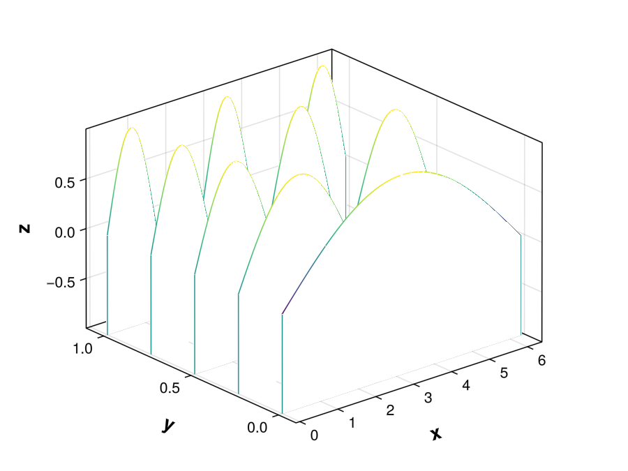
1.3 Waterfall plot

A waterfall plot is a 3D plot with a partial curtain along the y-axis.

waterfall_plot

---

waterfall_plot(x, y, z; zmin = minimum(z), lw = 1.,
               colorline = :auto, colmap = :viridis, colorband = (:white, 1.),
               xlabel = "x", ylabel = "y", zlabel = "z", edge = true,
               axis_tight = false, xlim = [minimum(x), maximum(x)],
               ylim = [minimum(y), maximum(y)], zlim = [zmin, maximum(z)])

Plot a waterfall plot.

Inputs

• x: x-axis values

• y: y-axis values

• z: z-axis values

• zmin: minimum value of z-axis

• lw::Real: linewidth

• colorline: color of the lines

• colmap: Name of the colormap

• colorband: Tuple defining the color of the band

  • color : Color

  • alpha : Alpha value for transparency

• xlabel: x-axis label

• ylabel: y-axis label

• zlabel: z-axis label

• edge: Display edges (default: true)

• axis_tight: Tight axis (default: false)

• xlim: x-axis limits

• ylim: y-axis limits

• zlim: z-axis limits

Output

• fig: Figure

x = range(0., 2π, 100)
y = range(0., 1., 5)

nx = length(x)
ny = length(y)
z = zeros(ny, nx)

for i in eachindex(y)
    z[i, :] = sin.(i*x/2.)
end

waterfall_plot(x, y, z, xlim = [-0.1, 2π + 0.1], ylim = [-0.1, 1.1])

1.4 Stabilization plot

The stabilization plot is used in the context of the modal analysis to plot the Stabilization diagram.

stabilization_plot

---

stabilization_plot(stab::StabilizationAnalysis, indicator; display_poles)

Plot stabilization diagram for EMA-MDOF pole stability analysis.

Inputs

• stab: EMA-MDOF stabilization data

• indicator: Indicator to plot

  • :psif : Power spectrum indicator function (default)

  • :cmif : Complex mode indicator function

• display_poles: Vector of Bool to choose which poles to display

  • display_poles[1] : Stable in frequency and damping (default: true)

  • display_poles[2] : Stable in frequency but not stable in damping (default: true)

  • display_poles[3] : Not stable in frequency (default: true)

Output

• fig: Figure

Examples of stabilization plot can be found in the Modal extraction documentation.

1.5 Peaks plot

The peaks plot is used to visualize the peak detection of a given function. It is a useful tool to define the parameters of the peak detection algorithm use to extract the poles using Sdof methods.

peaks_plot

---

peaks_plot(x, y; width = 5, min_prom = 0., max_prom = Inf,
          xlabel = "x", ylabel = "y")

Plot data with detected peaks.

Inputs

• x: x-axis values

• y: y-axis values

• width: Half-width of the peaks (default: 1)

• min_prom: Minimum peak prominence (default: 0.)

• max_prom: Maximum peak prominence (default: Inf)

• xlabel: x-axis label

• ylabel: y-axis label

Output

• fig: Figure

• pks: Detected peaks

# Signal used in Peaks.jl package documentation
T = 1/25
t = 0:T:23

y = 3sinpi.(0.1t) + 2sinpi.(0.2t) + sinpi.(0.6t)
peaks_plot(t, y)

Note

StructuralVibration.jl uses the Peaks.jl package for peak detection. This package includes the functions plotpeaks and peaksplot for visualizing peaks and their properties, such as prominence and width. These functions require that the peak detection has been performed beforehand.

The peaks_plot function in StructuralVibration.jl is a simplified version that provides a plotting function which first estimates the peaks and then plots the peaks.

1.6 SV plot

The SV plot (for StructuralVibration plot) is a general function for 2D plotting. It is a helper function aiming at simplifying the plotting process.

sv_plot

---

sv_plot(x, y...; lw = 1., xscale = identity, yscale = identity,
        axis_tight = true, title = " ", xlabel = "x", ylabel = "y",
        legend = (active = false, position = :right, orientation = :vertical, entry = " "))

Plot a 2D plot.

Inputs

• x: x-axis values

• y: y-axis values

• lw: linewidth

• xscale: x-axis scale (default: identity)

• yscale: y-axis scale (default: identity)

• axis_tight: Tight axis (default: true)

• title: Title of the plot (default: " ")

• xlabel: x-axis label

• ylabel: y-axis label

• legend: Legend parameters

  • active : Bool

  • position : Symbol

  • entry : String

Output

• fig: Figure

x_sv = range(0., 2π, 100)
z_sv = ntuple(i -> sin.(i*x_sv/2), 5)

# SV plot
sv_plot(x_sv, z_sv..., lw = 2., legend = (active = true,))

2 Mesh manipulation

To access the mesh manipulation functions, you need to activate the SVMeshExt.jl extension by running the following command:

using Meshes

This extension provides functions for mesh manipulation, such as building a mesh from nodes and elements, detrending a plane or a mesh, visualizing a mesh, deforming a grid, and renumbering the element connectivity.

2.1 Building a mesh

The build_mesh function allows you to build a mesh from nodes and elements. The function takes as input the nodes and the elements of the mesh and returns a SimpleMesh object from Meshes.jl.

build_mesh

---

construct_mesh(nodes, elts)

Generate mesh points and connectivity from node coordinates and element connectivity.

Inputs

• nodes::Matrix{Float64}: The node coordinates.

• elts::Vector{Vector{Int}}: The element connectivity.

Outputs

• points::Vector{Point}: A list of mesh points.

• tris::Vector{Triangle}: A list of triangular elements.

• quads::Vector{Quadrangle}: A list of quadrilateral elements.

Notes

• This function is restricted to 2D meshes where elements are either triangles or quadrilaterals.

2.2 Detrending a plane or a mesh

The detrend_plane and detrend_mesh functions allow you to detrend a plane or a mesh, respectively. The detrending process implemented in detrend_plane consists in fitting a plane to the data and substracting the fitted plane from the data. The detrend_mesh function first removes the mean from the mesh and then applies the detrend_plane function to the each plane.

detrend_plane

---

detrend_plane(nodes, plane = :xy)

Remove the planar trend from a set of 3D points based on the specified plane.

Inputs

• nodes::Matrix{Float64}: The original node coordinates.

• plane::Symbol: The plane to detrend against (:xy, :xz, or :yz).

Outputs

• detrended_nodes::Matrix{Float64}: The detrended node coordinates.

detrend_mesh

---

detrend_mesh(nodes, elts)

Remove global trends from a mesh defined by node coordinates and element connectivity.

Inputs

• nodes::Matrix{Float64}: The original node coordinates.

• elts::Vector{Vector{Int}}: The element connectivity.

Outputs

• det_nodes::Matrix{Float64}: The detrended node coordinates.

• det_mesh::SimpleMesh: The detrended mesh.

2.3 Deforming a grid

The deformed_grid function allows you to deform a grid of points by applying a set of values to its nodes. This is useful, for instance, for visualizing the deformation or mode shapes of a structure.

deformed_grid

---

deformed_grid(nodes, displacements; scale_factor = 20)

Generate a deformed grid of points by applying displacements to the original node coordinates.

Inputs

• nodes::Matrix{Float64}: The original node coordinates.

• values::Matrix{Float64}: The values to apply to the nodes.

• scale_factor::Float64: A factor to scale the values (default is 20).

Outputs

• deformed_nodes::Vector{Point}: A list of deformed points.

2.4 Renumbering the element connectivity

The renumber_element_connectivity function allows you to renumber the element connectivity of a mesh. This is useful when the element connectivity is not consistent with the node numbering. Indeed, Meshes.jl implicitly states that the nodes in a mesh are numbered from 1 to the number of nodes, and that the element connectivity is defined accordingly. If this is not the case, the renumber_element_connectivity function can be used to renumber the element connectivity to be consistent with the node numbering.

renumber_element_connectivity

---

renumber_element_connectivity(elts, nodes_ID)

Renumber elements connectivity based on a given list of node IDs.

Inputs

• elts::Vector{Vector{Int}}: The original element connectivity.

• nodes_ID::Vector{Int}: The list of node IDs.

Outputs

• elts_new::Vector{Vector{Int}}: The renumbered element connectivity.

Notes

• This function assumes that each node ID in nodes_ID corresponds to a unique node in the original mesh and that the element connectivity in elts references these node IDs.

• The renumbering is necessary if the elements ID are not contiguous or if they do not start from 1, which can cause issues when using Meshes.jl for visualization or further processing.

3 Mesh visualization and animation

To access the mesh manipulation and animation functions, you need to activate the SVMeshExt.jl extension by running the following command:

using Meshes, CairoMakie

# or

using Meshes, GLMakie

This extension provides functions for visualizing and animating meshes.

3.1 Visualizing a mesh

The viz_mesh function allows you to visualize a static mesh.

viz_mesh

---

viz_mesh(mesh; xlabel, ylabel, zlabel, title, color, colormap, alpha, showsegments, segmentsize, segmentcolor, xlim, ylim, zlim)

Visualize a 3D mesh with customizable options.

Inputs

• mesh: The mesh to visualize.

• xlabel::String: Label for the x-axis (default is "x").

• ylabel::String: Label for the y-axis (default is "y").

• zlabel::String: Label for the z-axis (default is "z").

• title::String: Title of the plot (default is an empty string).

• color: Color mapping for the mesh (default is :white).

• colormap::Symbol: Colormap to use for coloring the mesh (default is :jet1).

• alpha::Real: Transparency level of the mesh (default is 0.5).

• showsegments::Bool: Whether to show element segments (default is true).

• segmentsize::Real: Size of the segments if shown (default is 0.5).

• segmentcolor: Color of the segments if shown (default is :black).

• xlim::Tuple{Real, Real}: Limits for the x-axis (default is no limits).

• ylim::Tuple{Real, Real}: Limits for the y-axis (default is no limits).

• zlim::Tuple{Real, Real}: Limits for the z-axis (default is no limits).

Output

• fig::Figure: The figure containing the visualized mesh.

3.2 Animating a mesh

The animate_mesh function allows you to animate a mesh by applying a set of values to its nodes. This is useful, for instance, for visualizing the deformation or mode shapes of a structure.

animate_mesh

---

animate_mesh(nodes, elts, values; title, xlabel, ylabel, zlabel, color, colormap, alpha, showsegments, scale_factor, frequency, framerate, filename, xlim, ylim, zlim)

animate_mesh(nodes, elts, values, x; xlabel, ylabel, zlabel, color, colormap, alpha, showsegments, unit_x, quantity_y, scale_factor, framerate, title_update_framerate, filename, xlim, ylim, zlim)

Create an animation of a deformed mesh.

Inputs

• nodes::Matrix{Real}: Original node coordinates.

• elts::Vector{Vector{Int}}: Element connectivity.

• values::VecOrMat{Real}: Values to apply to the nodes.

• x::AbstractVector{Real}: Parameter values corresponding to each set of values (e.g., time or frequency).

• title::String: Title of the animation (default is "Animated mesh").

• xlabel::String: Label for the x-axis (default is "x").

• ylabel::String: Label for the y-axis (default is "y").

• zlabel::String: Label for the z-axis (default is "z").

• color: Color mapping for the mesh (default is the values).

• colormap::Symbol: Colormap to use for coloring the mesh (default is :jet1).

• alpha::Real: Transparency level of the mesh (default is 1.0).

• showsegments::Bool: Whether to show element segments (default is true).

• segmentsize::Real: Size of the segments if shown (default is 0.5).

• segmentcolor: Color of the segments if shown (default is :black).

• scale_factor::Real: Factor to scale the values (default is 100).

• framerate::Int: Frame rate of the animation in frames per second (default is 35).

• frequency::Real: Frequency of the animated motion in Hz (default is framerate).

• title_update_framerate::Int: How often (in frames) to update the title of the animation (default is 10).

• filename::String: Name of the output video file (default is "animate_mesh.mp4").

• xlim::Tuple{Real, Real}: Limits for the x-axis (default is no limits).

• ylim::Tuple{Real, Real}: Limits for the y-axis (default is no limits).

• zlim::Tuple{Real, Real}: Limits for the z-axis (default is no limits).

Outputs

• Animation saved as a video file showing the deformed mesh over time.

Notes

• When values is a vector of values and frequency is specified, the animation simulates a harmonic motion of the mesh based on the provided values and frequency. This is useful for visualizing mode shapes or operational deflection shapes in structural vibration analysis.

• When values is a matrix and x is provided, the animation shows the evolution of the mesh deformation as a function of the parameter x, which can represent time, frequency, or any other relevant parameter. The title of the animation updates dynamically every 10 frames to reflect the current value of x.

3.3 Example

In this example, we will visualize the second mode shape of a simply supported plate.

3.3.1 Data generation

using LazyGrids

# Dimensions
Lp = 0.6
bp = 0.4
hp = 1e-3

# Material parameters
E = 2.1e11
ρ = 7800.
ν = 0.33

plate = Plate(Lp, bp, hp, E, ρ, ν)

3.3.2 Mesh creation

# Helper function to create a quadrilateral mesh
function create_quad_mesh(xp::Vector, yp::Vector, nx::Int, ny::Int)
    # Number of quadrangles
    n_quads = (nx - 1) * (ny - 1)
    quads = Vector{Vector{Int}}(undef, n_quads)

    quad_idx = 1
    for j in 1:(ny-1)
        for i in 1:(nx-1)
            # Indices of the nodes of the quadrangle in counter-clockwise order
            n1 = (j-1) * nx + i
            n2 = (j-1) * nx + i + 1
            n3 = j * nx + i + 1
            n4 = j * nx + i

            quads[quad_idx] = [n1, n2, n3, n4]
            quad_idx += 1
        end
    end

    return quads
end

# Create the mesh
nx = 10
ny = 10
x, y = ndgrid(range(0., Lp, nx), range(0., bp, ny))
xp = x[:]
yp = y[:]
zp = zeros(length(xp))

nodes = [xp yp zp]
elts = create_quad_mesh(xp, yp, nx, ny)
mesh = build_mesh(nodes, elts)

fig_mesh = viz_mesh(mesh, zlim = (-0.15, 0.15), title = "Mesh of the plate")

3.3.3 Visualization of the mode shape

# Compute the second mode shape
ms = sin.(2π*xp/Lp) .* sin.(π*yp/bp)

# Compute deformed grid
ms_deformed = zeros(3size(nodes, 1))
ms_deformed[3:3:end] .= ms

dpoints = deformed_grid(nodes, ms_deformed, 0.15)

fig_deformed = viz_mesh(SimpleMesh(dpoints, mesh.topology.connec), color = ms, colormap = :jet1, alpha = 1., zlim = (-0.2, 0.2), title = "Deformed mesh of the plate")

3.3.4 Animating the mode shape

animate_mesh(nodes, elts, ms_deformed, color = ms, scale_factor = 0.1, zlim = (-0.2, 0.2), title = "Second mode shape of a simply supported rectangular plate", framerate = 24, filename = "animated_plate.mp4")

4 Theming

StructuralVibration.jl provides a set of themes for the plotting functions. The themes are defined in the theme_choice function.

theme_choice

---

theme_choice(name::Symbol; fonts = Makie.theme(:fonts),
             titlesize = 20., labelsize = 18., ticklabelsize = 14.)

Choose the theme for the plots.

Inputs

• name: Name of the theme

  • :makie

  • :sv

• fonts: Fonts of the figure (default: Makie.theme(:fonts))

• titlesize: Title size (default: 20.)

• labelsize: Label size (default: 18.)

• ticklabelsize: Tick label size (default: 14.)

Output

• theme: Theme

with_theme(theme_choice(:makie)) do
    sv_plot(x_sv, z_sv..., lw = 2., legend = (active = true,), title = ":makie theme")
end

with_theme(theme_choice(:makie)) do
    sv_plot(x_sv, z_sv..., lw = 2., legend = (active = true,), title = ":sv theme")
end