The modal approach enables the dynamic behavior of a structure to be predicted based on knowledge of its natural modes of vibration, which are intrinsic to the system. From a practical point of view, this information can be used to determine the frequencies at which the structure is most likely to vibrate. For industry, this information is invaluable, as vibrations can cause discomfort, noise, premature wear and tear, or even damage to a system. This is where Experimental Modal Analysis (EMA) comes in Experimental identification of vibration modes can also be used to calibrate a finite element model or certify a product (e.g. ground vibration testing or regulations related to the modal behavior of the structure).
EMA aims to estimate the natural frequencies of the system and other characteristic parameters (e.g. damping ratios and mode shapes) from the vibration measurements in order to obtain a modal model of the system under consideration. This model can then be used to determine the structure’s dynamic behaviour for a given excitation.
To reach these goals, it is supposed that:
the system is linear and time-invariant ;
the modal damping is of viscous type.
EMA is a family of inverse methods attempting to determine the modal characteristics of a structure from the responses measured at each point of the mesh.
1 General principles
To identify the modal parameters of a structure or mechanical system, EMA relies on the measurement of the structure’s transfer function matrix. By definition, the transfer function \(H_{pq}(\omega)\) can be seen as the frequency response of the system at a point \(x_p\) to an excitation of unit amplitude at a point \(x_q\). Classically, the transfer function matrix (here the admittance) is given by the relation
\(\lambda_i = -\xi_i\omega_i + j\,\Omega_i\) is the pole related to the mode \(i\), with:
\(\omega_i = \vert \lambda_i\vert\) is the natural angular frequency of the system
\(\Omega_i = \omega_i\sqrt{1 - \xi_i^2}\) is the damped natural frequency of the mode \(i\)
\(\xi_i = -\frac{\text{Re}(\lambda_i)}{\omega_i}\) the modal damping factor of the mode \(i\)
\({}_i R_{pq} = c_i\, \phi_i(x_p)\, \phi_i(x_q)\) is the residue of the mode \(i\), with:
\(\phi_i(x_p)\) the mode shape of the mode \(i\) at point \(x_p\)
\(c_i = \frac{1}{2jM_i\Omega_i}\) the normalization constant of the mode shape of the mode \(i\)
The objective of an EMA is therefore to identify the residuals \({}_i R_{pq}\) and the poles \(\lambda_i\) of the transfer function \(H_{pq}(\omega)\) in order to extract, in a second step, the modal parameters of the system under study (natural angular frequencies \(\omega_i\), modal damping factors \(\xi_i\) and mode shapes \(\phi_i\)).
In StructuralVibration.jl, two families of modal extraction methods are implemented:
methods based on the use of single degree of freedom (sdof) models, known as Sdof methods. These methods seek to adjust ideal transfer functions of Sdof systems to experimental curves around their resonances. These methods therefore consist of identifying the modal parameters mode by mode. To do this, the operator must select a frequency band around each resonance to perform the extraction.
methods based on the use of multiple degree of freedom (mdof) models, known as Mdof methods. These methods consider that the system can be represented as a multiple degree of freedom system. They are generally based on the construction of a high-order polynomial matrix whose coefficients are estimated from the measured transfer functions.
2 Sdof methods
The Sdof methods are based on the assumption that the system can be represented as a single degree of freedom system. This means that the system can be described by a single natural frequency, damping ratio, and mode shape. The Sdof methods are typically used for systems that are lightly damped and for which the modes are well separated.
For these methods, it is assumed that the FRF (admittance) is given by: \[
H_{pq}(\omega) = \sum_{i = 1}^N\frac{_{i}R_{pq}}{\omega_i^2 - \omega^2 + j\eta_i\omega_i^2}
\] where, for a mode \(i\), \(_{i}R_{pq} = \phi_i(x_p)\phi_i(x_q)\) is the residue, \(\omega_i\) is the natural frequency, \(\eta_i\) is the modal damping factor, and \(\phi_i(x_p)\) is the mass-normalized mode shape at the point \(x_p\).
When the natural frequencies of the modes are sufficiently spaced and the damping is low, one can write at a frequency \(\omega\) close to the natural frequency \(\omega_i\): \[
H_{pq}(\omega) \approx \frac{\phi_i(x_p)\phi_i(x_q)}{\omega_i^2 - \omega^2 + j\eta_i\omega_i^2}.
\]
Note
One can note that the modal damping factor \(\eta_i\) is related to the damping ratio \(\xi_i\) by the relation: \[
\eta_i = 2\xi_i.
\]
2.1 Poles extraction
StructuralDynamics.jl provides three SDOF methods for extracting the poles of a system from its frequency response function (FRF):
Peak picking method
Circle fit method
Least squares fit method
2.1.1 Peak picking method
The peak picking method is a simple and effective way to extract the natural frequencies and damping ratios of a system. The method consists of the following steps:
Identification of natural frequencies
They are identified from the peaks of the amplitude of the FRF. The natural frequencies are identified as the frequencies at which the FRF has a local maximum. The local maxima are determined using Peaks.jl.
To check the peak detection, one can use the peaksplot function from StructuralVibration.jl (see Peaks plot for more details).
Estimation of modal damping factors
To estimate the value of the damping factor for mode \(i\), the half power bandwidth method is used. This procedure, valid for low damping (\(\eta_i < 0.1\)), first determines the frequencies \(\omega_1\) and \(\omega_2\) such that: \[
\vert H_{pq}(\omega_1)\vert = \vert H_{pq}(\omega_2)\vert = \frac{\vert H_{pq}(\omega_i)\vert}{\sqrt{2}},
\] with \(\omega_i \in [\omega_1, \omega_2]\).
Knowing the values of \(\omega_i\), \(\omega_1\), and \(\omega_2\), the damping ratio for mode \(i\) is determined using the formula: \[
\eta_i = \frac{\omega_2^2 - \omega_1^2}{2\omega_i^2}.
\]
Note
If we consider that the shape of a resonance peak is symmetric then \(\omega_i = \frac{\omega_1 + \omega_2}{2}\).
It comes that: \[
\omega_2^2 - \omega_1^2 \approx 2\omega_i(\omega_2 - \omega_1).
\]
Hence, the damping ratio can be approximated as: \[
\eta_i \approx \frac{\omega_2 - \omega_1}{\omega_i}.
\]
This formula is often given in textbooks when dealing with the half power bandwidth method.
Once the natural frequencies and damping ratios have been determined, the poles are recovered using the relation: \[
\lambda_i = -\xi_i \omega_i + j\omega_i\sqrt{1 - \xi_i^2}.
\]
Warning
Thanks to its extreme simplicity, this method allows for quick analysis. However, this method generally does not provide satisfactory results, as it relies on measuring the resonance peak, which is very difficult to measure precisely. This is why this method is mainly applicable to lightly damped structures with well-separated modes, whose transfer functions have been measured with good frequency resolution.
2.1.2 Circle fit method
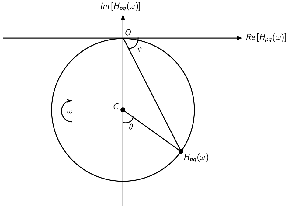
The circle fit method is a more sophisticated method for extracting the natural frequencies and damping ratios of a system. It allows for more accurate results than the peak picking method. It is based on the fact that the admittance forms a circle (Nyquist circle) when plotted in the complex plane (see Figure 1). Indeed, assuming that the modes are mass-normalized, it can be shown that: \[
Re\left[H_{pq}(\omega)\right]^2 + \left(Im\left[H_{pq}(\omega)\right] + \frac{\Phi_i(x_p)\Phi_i(x_q)}{2\eta_i\omega_i^2}\right)^2 = \left(\frac{\Phi_i(x_p)\Phi_i(x_q)}{2\eta_i\omega_i^2}\right)^2,
\] which is the equation of a circle of radius \(R = \frac{\vert\Phi_i(x_p)\Phi_i(x_q)\vert}{2\eta_i\omega_i^2}\) and center \((x_c,y_c) = \Bigl(0,-\frac{\Phi_i(x_p)\Phi_i(x_q)}{2\eta_i\omega_i^2}\Bigr)\).
Figure 1: Typical Nyquist circle of an admittance \(H_{pq}(\omega)\)
The circle fit method consists of the following steps:
Identification of natural frequencies
To identify the natural frequency of a mode \(i\), we start by parameterizing the Nyquist circle by defining the angles \(\psi\) and \(\theta\) as shown in Figure 1. Mathematically, it can then be shown that: \[
\omega_i^2 = \frac{\omega_1^2\tan\frac{\theta_2}{2} - \omega_2^2\tan\frac{\theta_1}{2}}{\tan\frac{\theta_2}{2} - \tan\frac{\theta_1}{2}},
\] where \(\omega_1\) and \(\omega_2\) are the angular frequencies such that \(\omega_1 < \omega_i < \omega_2\), while \(\theta_1\) and \(\theta_2\) are the corresponding angles of the Nyquist circle.
Estimation of modal damping factors
The damping ratio is estimated using the following formula: \[
\eta_i = \frac{\omega_2^2 - \omega_1^2}{\omega_i^2}\frac{1}{\tan\frac{\theta_1}{2} - \tan\frac{\theta_2}{2}}.
\]
Note
Generally, the angles \(\theta_1\) and \(\theta_2\) are chosen so that: \[
\theta_1 = \frac{\pi}{2} \text{ and } \theta_2 = -\frac{\pi}{2}.
\]
In doing so, we have: \[
\omega_i^2 = \frac{\omega_1^2 + \omega_2^2}{2} \text{ and } \eta_i = \frac{\omega_2^2 - \omega_1^2}{2\omega_i^2}.
\]
2.1.3 Least squares fit method
The least squares fit method is based on the idea of fitting the frequency response function (FRF) around the resonance peaks using a least squares approach1.
When the natural frequencies of the modes are sufficiently spaced and the damping is low, one can write at a frequency \(\omega\) close to the natural frequency \(f_i\): \[
H_{pq}(f) \approx \frac{{}_i A_{pq}}{f_i^2 - f^2 + 2j\xi_i f_i f}.
\]
The least squares fit method consists of the following steps:
Definition of the system matrices
To construct the system matrices, we start by rewriting the previous equation as: \[
H_{pq}(f) \left(f_i^2 - f^2 + 2j\xi_i f_i f\right) - {}_i A_{pq} = 0.
\]
This equation can be rewritten as: \[
\begin{bmatrix}
H_{pq}(f) & 2jfH_{pq}(f) & -1
\end{bmatrix} \begin{bmatrix}
f_i^2 \\
\xi_i f_i \\
_{i}A_{pq}
\end{bmatrix} = f^2 H_{pq}(f).
\]
If we consider \(M\) frequency points around the resonance peak, we can construct the following system of equations: \[
\begin{bmatrix}
H_{pq}(f_1) & 2jf_1H_{pq}(f_1) & -1 \\
H_{pq}(f_2) & 2jf_2H_{pq}(f_2) & -1 \\
\vdots & \vdots & \vdots \\
H_{pq}(f_M) & 2jf_MH_{pq}(f_M) & -1
\end{bmatrix} \begin{bmatrix}
f_i^2 \\
\xi_i f_i \\
_{i}A_{pq}
\end{bmatrix} = \begin{bmatrix}
f_1^2 H_{pq}(f_1) \\
f_2^2 H_{pq}(f_2) \\
\vdots \\
f_M^2 H_{pq}(f_M)
\end{bmatrix}.
\]
Least squares solution
The least squares solution of the previous system of equations is given by: \[
\begin{bmatrix}
f_i^2 \\
\xi_i f_i \\
_{i}A_{pq}
\end{bmatrix} = \left(\mathbf{A}^H\mathbf{A}\right)^{-1}\mathbf{A}^H\mathbf{b},
\] where \(\mathbf{A}\) is the matrix on the left-hand side of the system of equations, \(\mathbf{b}\) is the vector on the right-hand side, and \(\mathbf{A}^H\) is the conjugate transpose of \(\mathbf{A}\).
Note
In practice, the least squares solution is not directly computed using complex numbers, as this can lead to numerical issues. Instead, the only the real part is used to solve a real system of the same size.
2.1.4 Practical considerations
When using Sdof methods for modal parameter extraction, the detection of the resonance peaks is a crucial step. The accuracy of the extracted modal parameters heavily depends on the correct identification of these peaks. It is therefore recommended to visually inspect the detected peaks using the peaks_plot function from StructuralVibration.jl to ensure that they correspond to actual resonances in the FRF.
Internally, poles_extraction functions use the Peaks.jl package for peak detection. The parameters for peak detection (such as minimum prominence and width) can be adjusted to improve the accuracy of peak identification. In this functions, the average FRF amplitude across all measurement points converted in dB scale, i.e. \(\bar{H}(f) = 20 \log_{10} \left( \frac{1}{n_o n_i} \sum_{o=1}^{n_o} \sum_{i=1}^{n_i} |H_{oi}(f)| \right)\), is used for peak detection.
It results that when using peaks_plot, it is recommended to display \(\bar{H}(f)\) to be consistent with the peak detection performed in poles_extraction.
2.2 Mode shape extraction
The mode shapes are extracted from the admittance matrix at the resonance frequency \(\omega_i\). In this situation, the admittance matrix is defined as: \[
\mathbf{H} = \frac{1}{j\eta_i\omega_i^2}
\begin{bmatrix}
\Phi_i(x_1)^2 & \Phi_i(x_1)\Phi_i(x_2) & \ldots\ & \Phi_i(x_1)\Phi_i(x_N) \\
\Phi_i(x_2)\Phi_i(x_1) & \Phi_i(x_2)^2 & & \Phi_i(x_2)\Phi_i(x_N) \\
\vdots & & \ddots & \vdots \\
\Phi_i(x_N)\Phi_i(x_1) & \ldots & \ldots & \Phi_i(x_N)^2
\end{bmatrix},
\]
where \(\omega_i\) and \(\eta_i\) have been determined using the peak picking method or the circle fit method.
To determine the mode shapes from the knowledge of a column \(q\) (or a row \(p\)), proceed as follows:
From the measurement of an input admittance (diagonal term of the admittance matrix), the mode shape value at point \(x_q\) is obtained: \[
\Phi_i(x_q)^2 = -\eta_i\omega_i^2 \text{Im}(H_{qq}(\omega_i)).
\]
From the cross-admittances (off-diagonal terms of the admittance matrix), the mode shape value at a point \(x_p\) is calculated: \[
\Phi_i(x_p)\Phi_i(x_q) = -\eta_i\omega_i^2 \text{Im}(H_{pq}(\omega_i))
\]
3 Mdof methods
The Mdof methods are based on the assumption that the system can be represented as a multiple degree of freedom system. They are generally based on the construction of a high-order polynomial matrix whose coefficients are estimated from the measured FRFs. As for the SDOF methods, the estimation of the modal parameters is divided into two steps:
estimation of the poles of the system to extract the natural frequencies and modal damping ratios,
estimation of the residues to extract the mode shapes.
3.1 Poles extraction
The poles of the system are then obtained as the roots of the characteristic polynomial associated with this polynomial matrix. Three methods are implemented in this package:
the Least-Squares Complex Exponential (LSCE) method
the Least-Squares Complex Frequency-domain (LSCF) method
the Polyreference Least-Squares Complex Frequency-domain (pLSCF) method
3.1.1 LSCE method
The LSCE method is based on the assumption that the system can be modeled as a sum of complex exponentials in the time domain. The impulse response function (IRF) between an output \(o\) (\(o = 1, \ldots, n_o\)) and an input \(i\) (\(i = 1, \ldots, n_i\)) can be modeled as: \[
h_{oi}(t) = \sum_{k = 1}^n \left(c_k e^{\lambda_k t} + c_k^\ast e^{-\lambda_k^\ast t}\right) = 2 Re\left(\sum_{k = 1}^n c_k e^{\lambda_k t}\right).
\]
When sampling the IRF at a sampling period \(T_s\), one obtains the following discrete-time model: \[
h_{oi}[m] = 2 Re\left(\sum_{k = 1}^n c_k z_k^m\right) \text{ with } z_k = e^{\lambda_k T_s},
\]
for \(m = 0, 1, \ldots, 2n\), (\(n\) is the model order). According to the Prony’s method, the poles \(\lambda_k\) can be calculated from the roots of the following characteristic polynomial: \[
\sum_{m = 0}^{2n} \beta_m z_k^m = 0 \text{ with } \beta_{2n} = 1.
\]
The coefficients \(\beta_l\) of the characteristic polynomial can be estimated from the sampled IRF \(h_{oi}[m]\). Todo so, one first multiply \(h_{oi}[m]\) by the corresponding coefficients \(\beta_m\) and then sums the resulting equations for \(m = 0, 1, \ldots, 2n\). This leads to the following homogeneous set of equations: \[
\sum_{m = 0}^{2n} \beta_m h_{oi}[m] = 2 Re\left(\sum_{k = 1}^{n} c_k \sum_{m = 0}^{2n} \beta_m z_k^m\right).
\]
When \(z_k\) is a root of the characteristic polynomial, the right-hand side of the previous equation is equal to zero. Therefore, one can estimate the coefficients \(\beta_m\) by solving the following set of linear equations: \[
\sum_{m = 0}^{2n} \beta_m h_{oi}[m] = 0.
\]
The previous equation can be derived using different set of data points, \(h_{oi}[m]\), \(h_{oi}[m+1]\), \(\ldots\), \(h_{oi}[m + 2n]\) to obtain an overdetermined set of linear equations that can be solved in the least-squares sense2. In this package, the coefficients \(\beta_m\) are estimated by solving the following set of equations: \[
\begin{bmatrix}
h_{oi}[0] & h_{oi}[1] & \ldots & h_{oi}[2n-1] \\
h_{oi}[1] & h_{oi}[2] & \ldots & h_{oi}[2n] \\
\vdots & \vdots & \ddots & \vdots \\
h_{oi}[2n-1] & h_{oi}[2n] & \ldots & h_{oi}[4n-2]
\end{bmatrix}
\begin{bmatrix}
\beta_0 \\
\beta_1 \\
\vdots \\
\beta_{2n-1}
\end{bmatrix}
= -\begin{bmatrix}
h_{oi}[2n] \\
h_{oi}[2n+1] \\
\vdots \\
h_{oi}[4n-1]
\end{bmatrix}
\]
Once the coefficients \(\beta_m\) are estimated, the poles \(\lambda_k\) can be obtained from the roots \(z_k\) of the characteristic polynomial.
3.1.2 LSCF method
According to Guillaume et al. 3, the transfer function between an output \(o\) (\(o = 1, \ldots, n_o\)) and an input \(i\) (\(i = 1, \ldots, n_i\)) can be modeled in the frequency domain as: \[
\widehat{H}_k(\omega) = \frac{N_k(\omega)}{d(\omega)},
\]
where \(k = 1, \ldots, n_o n_i\) (\(k = (o - 1) n_i + i\)). Here, \(N_k(\omega)\) is the \(k\)-th element of the numerator matrix defined as: \[
N_k(\omega) = \mathbf{\Omega}(\omega)^T \boldsymbol{\beta}_k,
\]
while \(d(\omega)\) is the common denominator polynomial defined as: \[
d(\omega) = \mathbf{\Omega}(\omega)^T \boldsymbol{\alpha}.
\]
In the previous equations, \(\mathbf{\Omega}(\omega)\) is the vector of polynomial basis functions defined as: \[
\mathbf{\Omega}(\omega)^T = [1, \Omega_1(\omega), \ldots, \Omega_n(\omega)] \text{ with } \Omega_n(\omega) = \exp(-i\omega n T_s),
\]
where \(n\) is the order of the denominator polynomial (a.k.a the model order) and \(T_s\) is the sampling period. The vectors \(\boldsymbol{\beta}_k\) and \(\boldsymbol{\alpha}\) contain the coefficients of the numerator and denominator polynomials, respectively.
Based on the previous formulation of the FRFs, the LSCF method consists in estimating the coefficients of the numerator \(\boldsymbol{\beta}_k\) and denominator \(\boldsymbol{\alpha}\) polynomials by minimizing the following functional: \[
J(\boldsymbol{\theta}) = \sum_{k=1}^{n_o n_i} \sum_{j=1}^{n_f} \left| W_k(\omega_j)\left[H_k(\omega_j) d(\omega_j) - N_k(\omega_j)\right] \right|^2,
\]
where \(\boldsymbol{\theta} = [\boldsymbol{\beta}_1^T, \ldots, \boldsymbol{\beta}_{n_o n_i}^T, \boldsymbol{\alpha}^T]^T\) is the vector of unknown parameters to be estimated, \(H_k(\omega_j)\) is the measured FRF at frequency \(\omega_j\), \(n_f\) is the number of frequency lines used for the identification and \(W_k(\omega_j)\) is an arbitrary weighting function. In the package, a unitary weighting function is used, i.e. \(W_k(\omega_j) = 1\).
The poles of the transfer function are obtained from the roots of the characteristic polynomial associated with the denominator polynomial \(d(\omega)\), which are computed after having estimated the coefficients \(\boldsymbol{\alpha}\) as the argument of the minimum of the functional \(J(\boldsymbol{\theta})\) (see Ref. [2] for details).
3.1.3 pLSCF method
The pLSCF method is an extension of the LSCF method that makes it possible to take into account multiple reference sensors simultaneously (see Ref. [3] for details). When using only one reference sensor, the pLSCF method is equivalent to the LSCF method.
In this approach, the transfer function \(\widehat{\mathbf{H}}_o(\omega) \in \mathbb{C}^{1 \times n_i}\) between an output \(o\) (\(o = 1, \ldots, n_o\)) and a set of \(n_i\) inputs can be modeled in the frequency domain as: \[
\widehat{\mathbf{H}}_o(\omega) = \mathbf{N}_o(\omega) \mathbf{D}(\omega)^{-1},
\]
where \(\mathbf{N}_o(\omega) \in \mathbb{C}^{1 \times n_i}\) is the numerator matrix defined as: \[
\mathbf{N}_o(\omega) = \mathbf{\Omega}(\omega)^T \boldsymbol{\beta}_o,
\]
while \(\mathbf{D}(\omega) \in \mathbb{C}^{n_i \times n_i}\) is the denominator matrix defined as: \[
\mathbf{D}(\omega) = \mathbf{\Omega}(\omega)^T \boldsymbol{\alpha}.
\]
Based on the previous formulation of the FRFs, the pLSCF method consists in estimating the coefficients of the numerator \(\boldsymbol{\beta}_o\) and denominator \(\boldsymbol{\alpha}\) polynomials. To this end, one defines the weighted error between the measured and modeled FRFs as: \[
\boldsymbol{\varepsilon}_o(\omega_j, \boldsymbol{\theta}) = W_o(\omega_j)\left[\mathbf{H}_o(\omega_j) \mathbf{D}(\omega_j) - \mathbf{N}_o(\omega_j)\right]
\]
Then, an error matrix \(\mathbf{E}_o(\boldsymbol{\theta}) \in \mathbb{C}^{n_f \times n_i}\) is constructed by stacking the weighted errors \(\boldsymbol{\varepsilon}_o(\omega_j, \boldsymbol{\theta}) \in \mathbb{C}^{1 \times n_i}\) for all frequency lines, that is: \[
\mathbf{E}_o(\boldsymbol{\theta}) = \begin{bmatrix}
\boldsymbol{\varepsilon}_o(\omega_1, \boldsymbol{\theta}) \\
\vdots \\
\boldsymbol{\varepsilon}_o(\omega_{n_f}, \boldsymbol{\theta})
\end{bmatrix}
\]
Finally, the coefficients of the numerator and denominator polynomials are estimated by minimizing the following functional: \[
J(\boldsymbol{\theta}) = \sum_{o=1}^{n_o} \Vert\mathbf{E}_o(\boldsymbol{\theta})\Vert^2.
\]
The poles of the transfer function are obtained from the characteristic polynomial associated with the denominator matrix \(\mathbf{D}(\omega)\), by computing the eigenvalues of the so-called companion matrix4.
3.1.4 Stabilization diagram
When carrying out an EMA, the main question that arises is how many modes (or, more precisely, poles) are contained within the frequency band of interest. Analyzing the frequency response functions (transfer functions) provides an initial estimate. However, it is difficult to distinguish between multiple or nearby modes.
The stabilisation diagram is a fundamental EMA tool as it provides a clear and concise presentation of the poles of the system under study. The idea is to adjust the transfer function model by increasing the number of poles and displaying the results on a graph. Broadly speaking, increasing the order of the model (i.e. the number of poles) causes the true vibration modes to converge to a stable value, whereas the numerical modes appear inconsistently or randomly on the graph. Thus, as the poles converge to stable ones, markers appear on the graph to indicate the identified poles, as the order of the model is gradually increased. The selection of poles is generally based on the stability of natural frequencies, modal damping and/or mode shapes, moving from a model order \(n\) to an order \(n + 1\). In this package, the stability of the natural frequencies and damping ratios is used to identify the physical poles of the system. The stability criterion is set to 1% for the natural frequencies and 5% for the damping ratios, following common practice in the EMA field.
In StructuralVibration.jl, the stabilization diagram can be obtained using the stabilization function along with any of the Mdof methods described above. The identified stable poles can then be visualized using the stabilization_plot function (see Stabilization plot). The stabilization function returns an StabilizationAnalysis structure that contains all the information related to the stabilization analysis, which allows the user to manually select the appropriate poles and to further analyze (e.g. by using quality and analysis indicators) and visualize the results.
3.2 Mode shape extraction
Once the poles of the system have been identified using one of the Mdof methods described above, the residues can be computed to extract the mode shapes. In this package, the residues are computed using a least-squares approach based on the formulation of the FRFs as a sum of rational functions. The FRF between an output \(p\) (\(p = 1, \ldots, n_o\)) and an input \(q\) (\(q = 1, \ldots, n_i\)) can be expressed as: \[
H_{pq}(\omega) = \sum_{i = 1}^n \left(\frac{{}_iR_{pq}}{j\omega - \lambda_i} + \frac{{}_iR_{pq}^\ast}{j\omega - \lambda_i^\ast}\right),
\]
where \(R_{k, pq}\) is the residue associated with the pole \(\lambda_k\).
At a frequency line \(\omega\), the previous equation can be rewritten in matrix form as: \[
H_{pq}(\omega) = \begin{bmatrix}
\frac{1}{j\omega - \lambda_1} & \ldots & \frac{1}{j\omega - \lambda_n} & \frac{1}{j\omega - \lambda_1^\ast} & \ldots & \frac{1}{j\omega - \lambda_n^\ast}
\end{bmatrix}
\begin{bmatrix}
{}_1R_{pq} \\
\vdots \\
{}_nR_{pq} \\
{}_1R_{pq}^\ast \\
\vdots \\
{}_nR_{pq}^\ast
\end{bmatrix}
\]
This system of equations can be solved in the least-squares sense to estimate the residues \({}_iR_{pq}\). This procedure is implemented in the mode_residues function.
From the estimated residues, the mode shapes can be extracted using the following relation: \[
{}_iR_{pq} = c_i \phi_{p,i} \phi_{q,i},
\]
where \(c_i\) is a scaling factor, \(\phi_{p,i}\) (resp. nd \(\phi_{q,i}\)) is the \(p\)-th (resp. \(q\)-th) component of the mode shape associated with the \(i\)-th mode.
To solve for the mode shapes, a collocated measurement is required, i.e. \(p = q\). Thus, the mode shape components can be obtained as: \[
\phi_{p,i} = \sqrt{\frac{{}_iR_{pp}}{c_i}} \; \text{ and } \; \phi_{q,i} = \frac{{}_iR_{pq}}{\sqrt{c_i\; {}_iR_{pp}}}.
\]
Here, the scaling factors \(c_i\) can be computed based on a normalization criterion. In this package, the scaling factors are computed such that the modal mass of each mode shape is equal to one (mass normalization). The mode shapes can then be extracted using the modeshape_extraction function.
At this stage, it is important to note that the mode shapes are complex-valued. If the modes are known to be real (after checking the Mode complexity indicators), a real-normalization transformation can be applied to the mode shapes5. Here, we adopt the widely used approach based on the computation of the phase angle that minimizes the imaginary part of the mode shape.
Given a complex mode shape \(\boldsymbol{\Psi}_i\), the real-normalized mode shape \(\bar{\boldsymbol{\Psi}}_i^{real}\) is obtained as:
\[
\bar{\boldsymbol{\Psi}}_i^{real} = \Re\left(\boldsymbol{\Psi}_i e^{-j\theta_i}\right),
\] where \(\theta_i\) is the phase angle between the real and imaginary parts of the mode shape. This angle is computed from the coefficient (gradient) of the straight line that best fits the points \((\Re(\Psi_k), \Im(\Psi_k))\) for. This procedure is implemented in the real_normalization function.
4 FRF reconstruction
From the identified modal parameters (poles and residues), it is possible to reconstruct the frequency response functions (FRFs) of the system under study using the frf_reconstruction function. This function implements the following relation for a number \(M\) of identified modes:
\(\lambda_i = -\xi_i + j\,\Omega_i\) is the pole related to the mode \(i\), with:
\(\Omega_i = \omega_i\sqrt{1 - \xi_i^2}\) is the damped natural frequency of the mode \(i\), with \(\omega_i = \vert \lambda_i\vert\).
\(\xi_i = -\frac{\text{Re}(\lambda_i)}{\omega_i}\) the modal damping factor of the mode \(i\)
\({}_i R_{pq} = c_i\, \phi_i(x_p)\, \phi_i(x_q)\) is the residue of the mode \(i\), with:
\(\phi_i(x_p)\) the mode shape of the mode \(i\) at point \(x_p\)
\(c_i = \frac{1}{2jM_i\Omega_i}\) the normalization constant of the mode shape of the mode \(i\)
In practice, however, the reconstructed FRF may not perfectly match the experimental FRF due to the unmodeled contribution of the modes outside the frequency range of interest. To account for this, it is common to include lower and upper residuals in the FRF reconstruction. This means that the admittance matrix can be expressed as: \[
H_{pq}(\omega) = \sum_{i = 1}^{M} \left[\frac{{}_i R_{pq}}{(j\omega - \lambda_i)} + \frac{{}_i R_{pq}^\ast}{(j\omega - \lambda_i^\ast)}\right] - \frac{L_{pq}}{\omega^2} + U_{pq},
\]
where \(L_{pq}\) and \(U_{pq}\) are the lower and upper residuals, respectively. These residuals can be computed using the compute_residuals function.
Note
Theoretically, the residuals can be computed in conjunction with the estimation of the residues using a least-squares approach. However, we observed that this often leads to inaccurate estimates of the residuals. Therefore, in StructuralVibration.jl, the computation of the residuals is performed separately after estimating the residues and poles.
Finally, when only real mode shapes are available, it is possible to compute the residues from the modal parameters using the mode2residues function. This function implements the following relation: \[
{}_i R_{pq} = c_i\, \phi_i(x_p)\, \phi_i(x_q),
\]
where \(\phi_i(x_p)\) is the mode shape of the mode \(i\) at point \(x_p\) and \(c_i = \frac{1}{2jM_i\Omega_i}\) is the normalization constant of the mode shape of the mode \(i\). Here, \(M_i = 1\), since the mode shapes are mass-normalized. during the extraction process. –>
5 API
Data types
EMAProblem
EMAProblem(frf, freq; frange, type_frf)
Data structure defining the inputs for EMA modal extraction methods.
Constructor parameters
frf::Array{Complex, 3}: 3D FRF matrix (array nm x ne x nf)
freq::AbstractArray{Real}: Vector of frequency values (Hz)
frange::Vector{Real}: Frequency range for analysis (default: [freq[1], freq[end]])
type_frf::Symbol: Type of FRF used in the analysis
:dis: Admittance (default)
:vel: Mobility
:acc: Accelerance
Fields
frf::Array{Complex, 3}: 3D admittance matrix (array nm x ne x nf)
freq::AbstractArray{Real}: Vector of frequency values (Hz)
type_frf::Symbol: Type of FRF used in the analysis
Note The FRF is internally converted to admittance if needed.
EMASolution
EMASolution(poles, ms, ci, res, lr, ur)
Structure containing the solution of the automatic experimental modal analysis using Mdof methods
Fields
poles::Vector{Complex}: Extracted poles
ms::AbstractArray{Real}: Mode shapes
ci::Vector{Complex}: Scaling constants for each mode
res::AbstractArray{Complex}: Residues for each mode
Data structure summarizing the results of the stabilization analysis.
Fields
prob::MdofProblem: EMA-MDOF problem containing FRF data and frequency vector
frange::Vector{Real}: Frequency range used for the stabilization analysis
poles::Vector{Vector{Complex}}: Vector of vectors containing extracted poles at each model order
modefn::Matrix{Real}: Matrix containing the natural frequencies (useful for plotting)
mode_stabfn::Matrix{Bool}: Matrix indicating the stability of natural frequencies
mode_stabdr::Matrix{Bool}: Matrix indicating the stability of damping ratios
Note
This structure is returned by the stabilization function after performing a stabilization diagram analysis and used by stabilization_plot for visualization.
PeakPicking
PeakPicking
Peak picking method for Sdof modal extraction
Fields
nothing
References
[1] D.J. Ewins, "Modal Testing: Theory, Practice and Application", 2nd Edition, Research Studies Press, 2000.
[2] D. J. Inman, "Engineering Vibration", 4th Edition, Pearson, 2013.
CircleFit
PeakPicking
Circle fitting method for Sdof modal extraction
Fields
nothing
References
[1] D.J. Ewins, "Modal Testing: Theory, Practice and Application", 2nd Edition, Research Studies Press, 2000.
[2] D. J. Inman, "Engineering Vibration", 4th Edition, Pearson, 2013.
LSFit
LSFit
Least squares fitting method for Sdof modal extraction
Fields
nothing
Reference
[1] A. Brandt, "Noise and Vibration Analysis: Signal Analysis and Experimental Procedures", Wiley, 2011.
LSCE
LSCE
Least Squares Complex Exponential method for Mdof modal extraction
Fields
nothing
Reference
[1] D. L. Brown, R. J. Allemang, Ray Zimmerman and M. Mergeay. "Parameter Estimation Techniques for Modal Analysis". SAE Transactions, vol. 88, pp. 828-846, 1979.
LSCF
LSCF
Least Squares Complex Frequency method for Mdof modal extraction
Fields
nothing
References
[1] P. Guillaume, P. Verboven, S. Vanlanduit, H. Van der Auweraer, and B. Peeters, "A poly-reference implementation of the least-squares complex frequency-domain estimator". In Proceedings of IMAC XXI. Kissimmee, FL, 2003.
[2] El-Kafafy M., Guillaume P., Peeters B., Marra F., Coppotelli G. (2012).Advanced Frequency-Domain Modal Analysis for Dealing with Measurement Noise and Parameter Uncertainty. In: Allemang R., De Clerck J., Niezrecki C., Blough J. (eds) Topics in Modal Analysis I, Volume 5. Conference Proceedings of the Society for Experimental Mechanics Series. Springer, New York, NY
pLSCF
pLSCF
Polyreference Least Squares Complex Frequency method for Mdof modal extraction
Fields
nothing
References
[1] P. Guillaume, P. Verboven, S. Vanlanduit, H. Van der Auweraer, and B. Peeters, "A poly-reference implementation of the least-squares complex frequency-domain estimator". In Proceedings of IMAC XXI. Kissimmee, FL, 2003.
[2] El-Kafafy M., Guillaume P., Peeters B., Marra F., Coppotelli G. (2012).Advanced Frequency-Domain Modal Analysis for Dealing with Measurement Noise and Parameter Uncertainty. In: Allemang R., De Clerck J., Niezrecki C., Blough J. (eds) Topics in Modal Analysis I, Volume 5. Conference Proceedings of the Society for Experimental Mechanics Series. Springer, New York, NY
max_prom::Real: Maximum peak prominence (only for Sdof methods, default: Inf)
pks_indices::Vector{Int}: Indices of peaks to consider (only for Sdof methods, default: empty vector)
Outputs
poles: Vector of extracted complex poles
Note
For Sdof methods, the natural frequencies and damping ratios are extracted from each FRF (each row of the matrix) and then averaged. The number of FRF used for averaging are those having the maximum (and same) number of peaks detected.
prob::EMAProblem: EMA problem containing FRF data and frequency vector
poles: Vector of complex poles
alg::SdofModalExtraction or alg::MdofEMA: Modal extraction algorithm
dpi: Driving point indices - default = [1, 1]
dpi[1]: Driving point index on the measurement mesh
dpi[2]: Driving point index on the excitation mesh
modetype: Type of mode shape (only for Mdof methods)
:emac: EMA - Complex mode shapes (default)
:emar: EMA - Real mode shapes
:oma: OMA
Output
ms: Mode shapes
ci: Scaling factors vector (only for Mdof methods)
Note
If the number of measurement points is less than the number of excitation points, the mode shapes are estimated at the excitation points (roving hammer test). Otherwise, the mode shapes are estimated at the measurement points (roving accelerometer test).
The alg argument is here for performing multiple dispatch but is not used in the function.
References [1] M. Géradin and D. J. Rixen. "Mechanical Vibrations: Theory and Application to Structural Dynamics". 3rd. Edition, Wiley, 2015.
[2] C. Ranieri and G. Fabbrocino. "Operational Modal Analysis of Civil Engineering Structures: An Introduction and Guide for Applications". Springer, 2014.
modal2poles
modal2poles(fn, ξn)
Convert natural frequencies and damping ratios to complex poles.
Inputs
fn: Vector of natural frequencies (Hz)
ξn: Vector of damping ratios
Output
poles: Vector of complex poles
poles2modal
poles2modal(poles)
Convert complex poles to natural frequencies and damping ratios.
Input
poles: Vector of complex poles
Outputs
fn: Vector of natural frequencies (Hz)
ξn: Vector of damping ratios
real_normalization
real_normalization(Ψ)
Converts the complex modes to real modes
Input
Ψ: Complex modes
Output
ϕn: Real modes
Reference
[1] E. Hiremaglur. "Real-Normalization of Experimental Complex Modal Vectors with Modal Vector Contamination". MS Thesis. University of Cincinnati, 2014.
# Computation of the mode residuesres_pp =mode2residues(ms_id, poles_pp, [2], 1:21)[1]# FRF reconstruction - without residualsH_sdof =frf_reconstruction(res_pp, poles_pp, freq)# FRF reconstruction - with residualslr, ur =compute_residuals(prob_sdof, res_pp, poles_pp)H_sdof2 =frf_reconstruction(res_pp, poles_pp, freq, lr = lr, ur = ur)
6.3 Mdof methods
6.3.1 Poles extraction
# EMA problemprob_mdof =EMAProblem(H, freq)# Poles extractionorder =10# Model orderp_lsce =poles_extraction(prob_mdof, order, LSCE())p_lscf =poles_extraction(prob_mdof, order, LSCF())p_plscf =poles_extraction(prob_mdof, order, pLSCF())# Stabilization diagram analysis using the LSCF methodstab =stabilization(prob_mdof, order, LSCF())# Visualization of the stabilization diagramstabilization_plot(stab)
6.3.2 Mode shape extraction
# Driving point indicesdpi = [1, 2]# Computation of the mode residuesres =mode_residues(prob_mdof, p_lscf)# Extraction of the mode shapesms_est =modeshape_extraction(res, p_lscf, LSCF(), dpi = dpi, modetype =:emar)[1]# Convert to real mode shapesms_est_real =real_normalization(ms_est)
6.3.3 FRF reconstruction
# Problem definitionprob_mdof =EMAProblem(H, freq)# Poles extraction using the Least-Squares Complex Frequency-domain methodpoles_lscf =poles_extraction(prob_mdof, 20, LSCF())# Residues extractionres_lscf =mode_residues(prob_mdof, poles_lscf)# FRF reconstruction - without residualsH_mdof =frf_reconstruction(res_lscf, poles_lscf, freq)# FRF reconstruction - with residualslr, ur =compute_residuals(prob_mdof, res_lscf, poles_lscf)H_mdof2 =frf_reconstruction(res_lscf, poles_lscf, freq, lr = lr, ur = ur)
Footnotes
A. Brandt. “Noise and Vibration Analysis: Signal Analysis and Experimental Procedures”, Wiley, 2011.↩︎
D. Brown, R. Allemang and R. Zimmerman and M. Mergeay. “Parameter estimation techniques for modal analysis”. SAE Technical Paper 790221, 1979.↩︎
P. Guillaume, P. Verboven, S. Vanlanduit, H. Van der Auweraer and B. Peeters, “A poly-reference implementation of the least-squares complex frequency-domain estimator”. Proceedings of the 21st International Modal Analysis Conference, IMAC, 2003.↩︎
M. El-Kafafy, P. Guillaume, B. Peeters, F. Marra, G. Coppotelli. “Advanced Frequency-Domain Modal Analysis for Dealing with Measurement Noise and Parameter Uncertainty”. In: Allemang R., De Clerck J., Niezrecki C., Blough J. (eds) Topics in Modal Analysis I, Volume 5. Conference Proceedings of the Society for Experimental Mechanics Series. 2012.↩︎
E. Hiremaglur. “Real-Normalization of Experimental Complex Modal Vectors with Modal Vector Contamination”. MS Thesis. University of Cincinnati, 2014.↩︎