Visualization extensions

StructuralVibration.jl is accompanied by an extension SVMakieExt.jl providing visualization capabilities. The extension provides a set of functions to visualize the results of the structural dynamics analysis.

To use one of these extensions, you need to import the desired plotting package by running the following command:

using CairoMakie

# or

using GLMakie

1 Bode plot

A Bode plot is a graph of the magnitude and phase of a transfer function versus frequency.

bode_plot

---

bode_plot(freq, y...; lw = 1., xlab = "Frequency (Hz)",
          ylab = "Magnitude (dB)", xscale = identity,
          axis_tight = true, isdeg = false, layout = :vertical,
          ref_dB = 1., legend = (active = false, position = :rt, entry = " "))

Plot Bode diagram of a frequency response or a FRF.

Inputs

• freq: Frequency range of interest

• y: Frequency response or FRF

• lw: Line width

• xlab: x-axis label

• xscale: x-axis scale (default: :log)

• axis_tight: Tight axis (default: false)

• isdeg: Phase in degrees (default: false)

• layout: Layout of the plot (default: :vertical)

• ref_dB: Reference value for magnitude (default: 1.)

• legend: Legend parameters (default: (active = false, position = :rt, entry = " "))

Output

• fig: Figure

# Initialize a Sdof type
m = 1.
f₀ = 10.
ξ = 0.01
sdof = Sdof(m, f₀, ξ)

# Computation parameters
freq = 1.:0.01:30.

# Compute the FRF
prob_frf = SdofFRFProblem(sdof, freq)
H = solve(prob_frf).u

# Bode plot
bode_plot(freq, H)

2 Nyquist plot

The Nyquist plot is either a 2D or 3D plot. In 2D, it is a graph of the imaginary part versus the real part of the transfer function. In 3D, it is a graph of the imaginary part versus the real part of the transfer function and the frequency.

2.1 2D plot

nyquist_plot

---

nyquist_plot(y)

Plot Nyquist diagram

Inputs

• y: Complex data vector

Output

• fig: Figure

nyquist_plot(H)

2.2 3D plot

nyquist_plot

---

nyquist_plot(freq, y, xlab = "Frequency (Hz)";
             projection = false)

Plot Nyquist diagram in 3D

Inputs

• freq: Frequency range

• y: Complex vector

• ylabel: y-axis label

• projection: Projection of the curve on the xy, yz, and xz planes (default: false)

  • on the xy plane: (freq, real(y))

  • on the yz plane: (imag(y), freq)

  • on the xz plane: (real(y), imag(y))

Output

• fig: Figure

nyquist_plot(freq, H, projection = true)

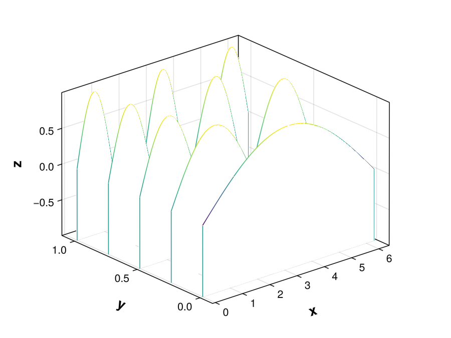
3 Waterfall plot

A waterfall plot is a 3D plot with a partial curtain along the y-axis.

waterfall_plot

---

waterfall_plot(x, y, z; zmin = minimum(z), lw = 1.,
               colorline = :auto, colmap = :viridis, colorband = (:white, 1.),
               xlabel = "x", ylabel = "y", zlabel = "z", edge = true,
               axis_tight = false, xlim = [minimum(x), maximum(x)],
               ylim = [minimum(y), maximum(y)], zlim = [zmin, maximum(z)])

Plot a waterfall plot.

Inputs

• x: x-axis values

• y: y-axis values

• z: z-axis values

• zmin: minimum value of z-axis

• lw::Real: linewidth

• colorline: color of the lines

• colmap: Name of the colormap

• colorband: Tuple defining the color of the band

  • color : Color

  • alpha : Alpha value for transparency

• xlabel: x-axis label

• ylabel: y-axis label

• zlabel: z-axis label

• edge: Display edges (default: true)

• axis_tight: Tight axis (default: false)

• xlim: x-axis limits

• ylim: y-axis limits

• zlim: z-axis limits

Output

• fig: Figure

x = range(0., 2π, 100)
y = range(0., 1., 5)

nx = length(x)
ny = length(y)
z = zeros(ny, nx)

for i in eachindex(y)
    z[i, :] = sin.(i*x/2.)
end

waterfall_plot(x, y, z, xlim = [-0.1, 2π + 0.1], ylim = [-0.1, 1.1])

4 SV plot

The SV plot (for StructuralVibration plot) is a general function for 2D plotting. It is a helper function aiming at simplifying the plotting process.

sv_plot

---

sv_plot(x, y...; lw = 1., xscale = identity, yscale = identity,
        axis_tight = true, title = " ", xlabel = "x", ylabel = "y",
        legend = (active = false, position = :right, orientation = :vertical, entry = " "))

Plot a 2D plot.

Inputs

• x: x-axis values

• y: y-axis values

• lw: linewidth

• xscale: x-axis scale (default: identity)

• yscale: y-axis scale (default: identity)

• axis_tight: Tight axis (default: true)

• title: Title of the plot (default: " ")

• xlabel: x-axis label

• ylabel: y-axis label

• legend: Legend parameters

  • active : Bool

  • position : Symbol

  • entry : String

Output

• fig: Figure

x = range(0., 2π, 100)
z_sv = ntuple(i -> sin.(i*x/2), 5)

# SV plot
sv_plot(x, z_sv..., lw = 2., legend = (active = true,))

5 Theming

StructuralVibration.jl provides a set of themes for the plotting functions. The themes are defined in the theme_choice function.

theme_choice

---

theme_choice(name::Symbol; fonts = Makie.theme(:fonts),
             titlesize = 20., labelsize = 18., ticklabelsize = 14.)

Choose the theme for the plots.

Inputs

• name: Name of the theme

  • :makie

  • :sv

• fonts: Fonts of the figure (default: Makie.theme(:fonts))

• titlesize: Title size (default: 20.)

• labelsize: Label size (default: 18.)

• ticklabelsize: Tick label size (default: 14.)

Output

• theme: Theme

with_theme(theme_choice(:makie)) do
    sv_plot(x, z_sv..., lw = 2., legend = (active = true,), title = ":makie theme")
end

with_theme(theme_choice(:makie)) do
    sv_plot(x, z_sv..., lw = 2., legend = (active = true,), title = ":sv theme")
end