StructuralVibration.jl provides a set of applications for simulating the dynamic response of 1-DOF and 2-DOF systems. These applications are designed to help users understand the behavior of these systems under various conditions.
These applications are intended to be used as educational tools, allowing users to explore the effects of different parameters on the system’s response. The applications are defined as an extension SVAppsExt.jl.
Five applications are provided: - Free Response of a 1-DOF System: This application simulates the free response of a single degree of freedom system, allowing users to observe how the system behaves when it is displaced from its equilibrium position and then released.
Forced Response of a 1-DOF System: This application simulates the forced response of a single degree of freedom system, allowing users to observe how the system responds to an external force applied to it.
Free Response of a 2-DOF System: This application simulates the free response of a two degree of freedom system, allowing users to observe how the system behaves when it is displaced from its equilibrium position and then released.
Forced Response of a 2-DOF System: This application simulates the forced response of a two degree of freedom system, allowing users to observe how the system responds to an external force applied to it.
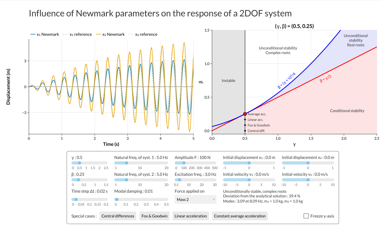
Newmark Method for a 2-DOF System: This application implements the Newmark method for simulating the response of a two degree of freedom system, allowing users to observe how the system responds to various parameters.
Free Response of a 1-DOF System
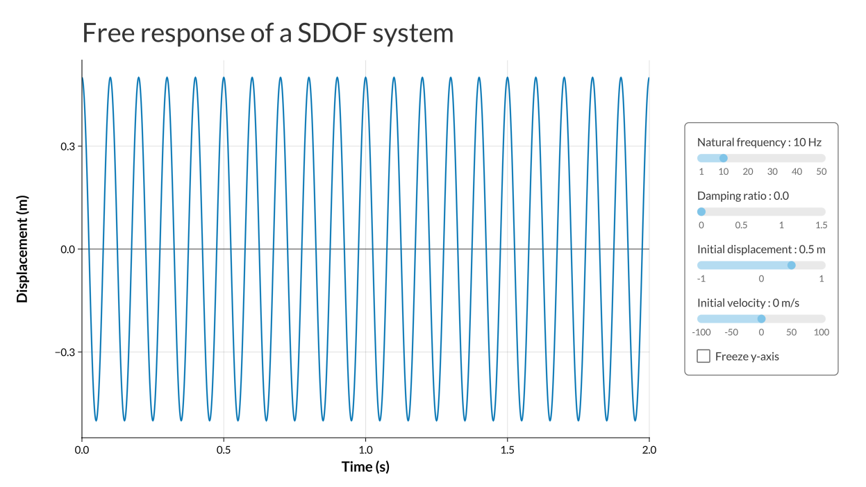
free_response_1dof
free_response_1dof(m = 1., t = 0.:1e-3:2.)
Launch an interactive application to visualize the free response of a single-degree-of-freedom (SDOF) system
Inputs
Output
Forced Response of a 1-DOF System
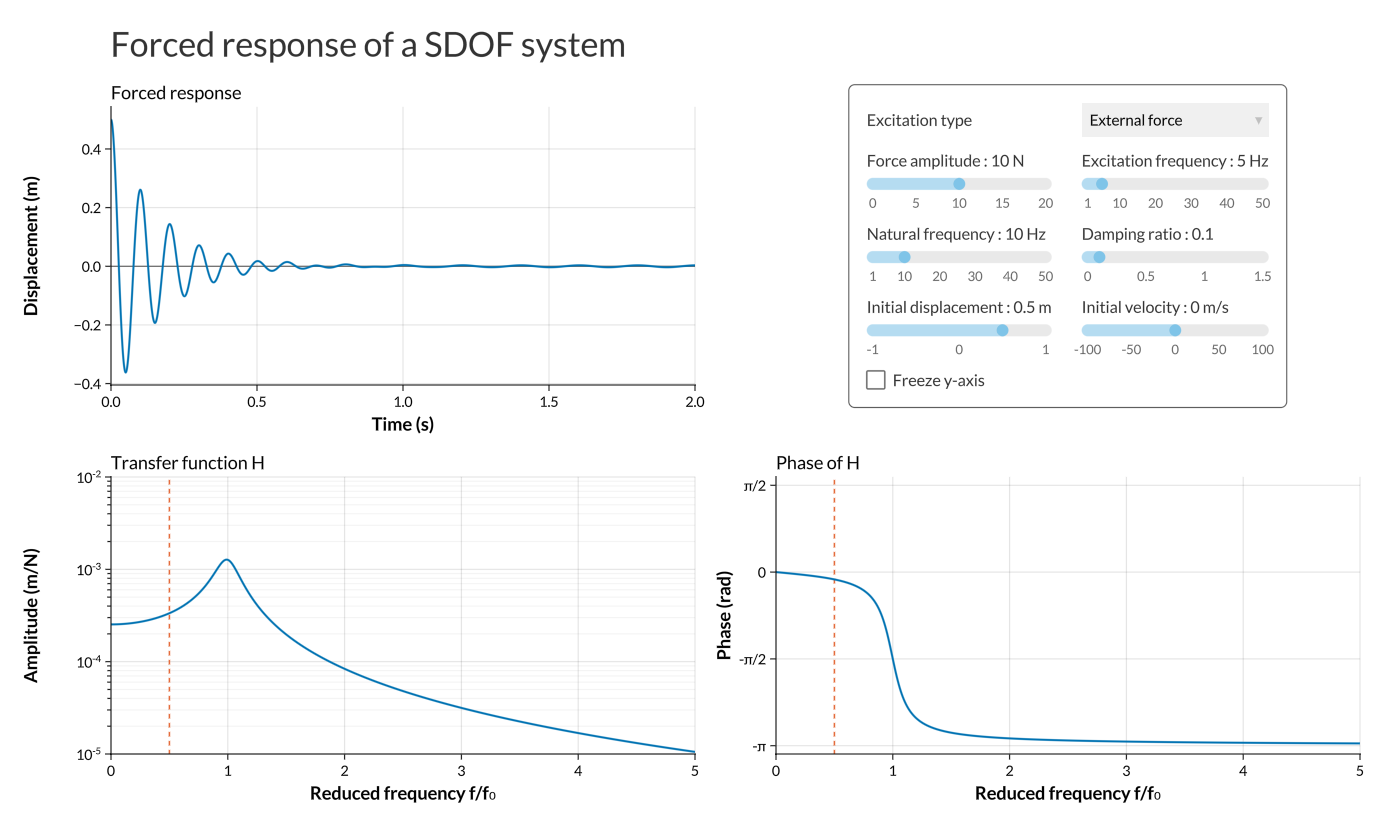
forced_response_1dof
forced_response_1dof(m, t, r, Fmax, xbmax)
Launch an interactive application to visualize the forced response of a single-degree-of-freedom (SDOF) system
Inputs
m: Mass of the system (default: 1.0)
t: Time vector (default: 0.:1e-3:2.)
r: Reduced frequency vector (default: 0.:0.005:5.)
Fmax: Maximum excitation force (default: 20.0)
xbmax: Maximum base displacement (default: 2.0)
Output
Free Response of a 2-DOF System
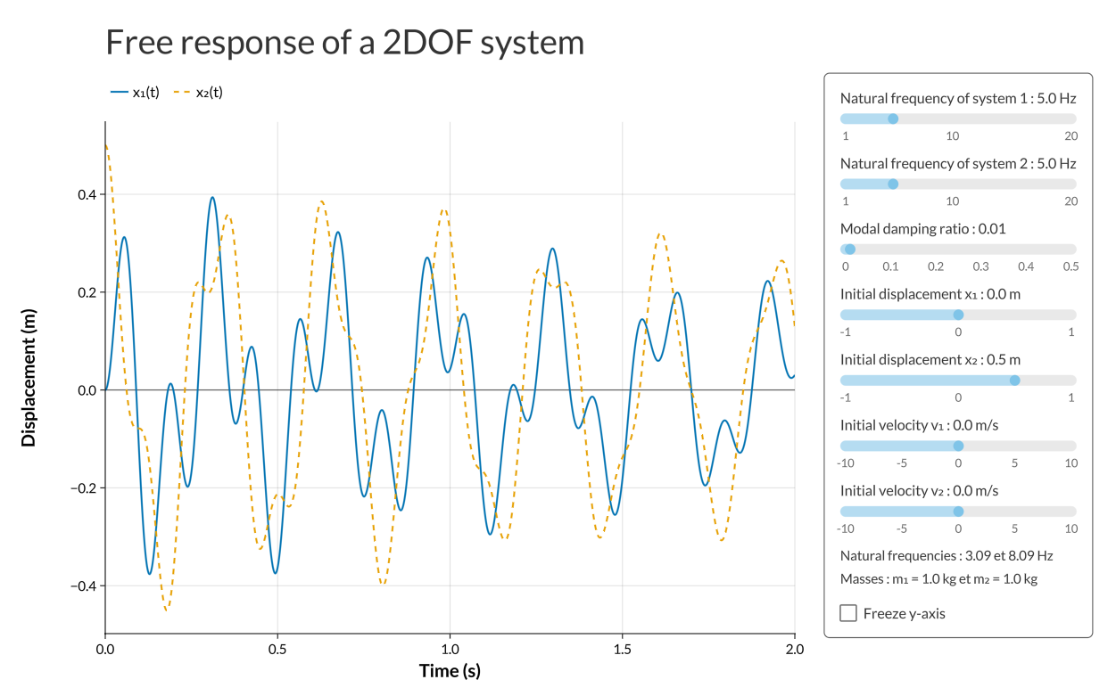
free_response_2dof
free_response_2dof(m1, m2, t)
Launch an interactive application to visualize the free response of a two-degree-of-freedom (2DOF) system
Inputs
m1: Mass of the first degree of freedom (default: 1.0)
m2: Mass of the second degree of freedom (default: 1.0)
t: Time vector over which the response is computed (default: 0.0 to 2.0 seconds with a step of 1e-3)
Output
Forced Response of a 2-DOF System
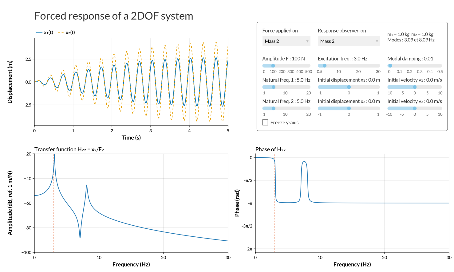
forced_response_2dof
forced_response_2dof(m1, m2, t, freq)
Launch an interactive application to visualize the forced response of a two-degree-of-freedom (2DOF) system
Inputs
m1: Mass of the first degree of freedom (default: 1.0)
m2: Mass of the second degree of freedom (default: 1.0)
t: Time vector over which the response is computed (default: 0.0 to 5.0 seconds with a step of 1e-3)
freq: Frequency vector over which the transfer function is computed (default: 0.0 to 30.0 Hz with a step of 0.01)
Output
Newmark Method for a 2-DOF System
newmark_2dof
newmark_2dof(m1, m2, t)
Launch an interactive application to visualize the influence of Newmark parameters on the response of a two-degree-of-freedom (2DOF) system
Inputs
m1: Mass of the first degree of freedom (default: 1.0)
m2: Mass of the second degree of freedom (default: 1.0)
t: Time vector over which the response is computed (default: 0.0 to 5.0 seconds with a step of 1e-3)
Output