The Sdof methods are based on the assumption that the system can be represented as a single degree of freedom system. This means that the system can be described by a single natural frequency, damping ratio, and mode shape. The Sdof methods are typically used for systems that are lightly damped and for which the modes are well separated.
For these methods, it is assumed that the FRF (admittance) is given by: \[
H_{pq}(\omega) = \sum_{i = 1}^N\frac{_{i}R_{pq}}{\omega_i^2 - \omega^2 + j\eta_i\omega_i^2}
\] where, for a mode \(i\), \(_{i}R_{pq} = \phi_i(x_p)\phi_i(x_q)\) is the residue, \(\omega_i\) is the natural frequency, \(\eta_i\) is the modal damping factor, and \(\phi_i(x_p)\) is the mass-normalized mode shape at the point \(x_p\).
When the natural frequencies of the modes are sufficiently spaced and the damping is low, one can write at a frequency \(\omega\) close to the natural frequency \(\omega_i\): \[
H_{pq}(\omega) \approx \frac{\phi_i(x_p)\phi_i(x_q)}{\omega_i^2 - \omega^2 + j\eta_i\omega_i^2}.
\]
Note
One can note that the modal damping factor \(\eta_i\) is related to the damping ratio \(\xi_i\) by the relation: \[
\eta_i = 2\xi_i.
\]
1 Poles extraction
StructuralDynamics.jl provides three SDOF methods for extracting the poles of a system from its frequency response function (FRF):
Peak picking method,
Circle fit method,
Least squares fit method.
1.1 Peak picking method
The peak picking method is a simple and effective way to extract the natural frequencies and damping ratios of a system. The method consists of the following steps:
Identification of natural frequencies
They are identified from the peaks of the amplitude of the FRF. The natural frequencies are identified as the frequencies at which the FRF has a local maximum. The local maxima are determined using Peaks.jl.
Estimation of modal damping factors
To estimate the value of the damping factor for mode \(i\), the half power bandwidth method is used. This procedure, valid for low damping (\(\eta_i < 0.1\)), first determines the frequencies \(\omega_1\) and \(\omega_2\) such that: \[
\vert H_{pq}(\omega_1)\vert = \vert H_{pq}(\omega_2)\vert = \frac{\vert H_{pq}(\omega_i)\vert}{\sqrt{2}},
\] with \(\omega_i \in [\omega_1, \omega_2]\).
Knowing the values of \(\omega_i\), \(\omega_1\), and \(\omega_2\), the damping ratio for mode \(i\) is determined using the formula: \[
\eta_i = \frac{\omega_2^2 - \omega_1^2}{2\omega_i^2}.
\]
Note
If we consider that the shape of a resonance peak is symmetric then \(\omega_i = \frac{\omega_1 + \omega_2}{2}\).
It comes that: \[
\omega_2^2 - \omega_1^2 \approx 2\omega_i(\omega_2 - \omega_1).
\]
Hence, the damping ratio can be approximated as: \[
\eta_i \approx \frac{\omega_2 - \omega_1}{\omega_i}.
\]
This formula is often given in textbooks when dealing with the half power bandwidth method.
Once the natural frequencies and damping ratios have been determined, the poles are recovered using the relation: \[
\lambda_i = -\xi_i \omega_i + j\omega_i\sqrt{1 - \xi_i^2}.
\]
Warning
Thanks to its extreme simplicity, this method allows for quick analysis. However, this method generally does not provide satisfactory results, as it relies on measuring the resonance peak, which is very difficult to measure precisely. This is why this method is mainly applicable to lightly damped structures with well-separated modes, whose transfer functions have been measured with good frequency resolution.
1.2 Circle fit method
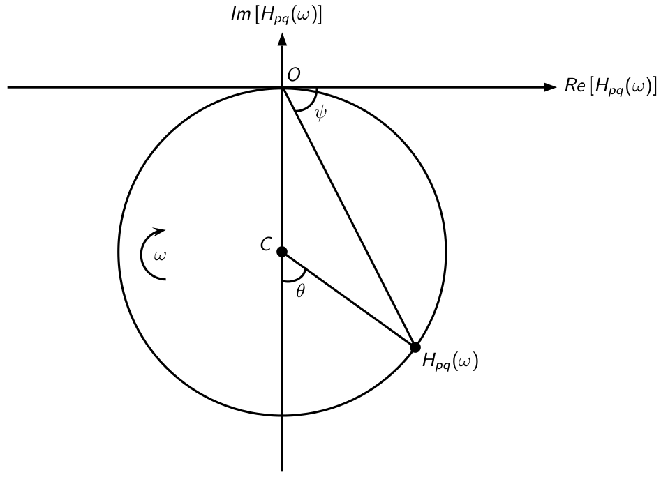
The circle fit method is a more sophisticated method for extracting the natural frequencies and damping ratios of a system. It allows for more accurate results than the peak picking method. It is based on the fact that the admittance forms a circle (Nyquist circle) when plotted in the complex plane (see Figure 1). Indeed, assuming that the modes are mass-normalized, it can be shown that: \[
Re\left[H_{pq}(\omega)\right]^2 + \left(Im\left[H_{pq}(\omega)\right] + \frac{\Phi_i(x_p)\Phi_i(x_q)}{2\eta_i\omega_i^2}\right)^2 = \left(\frac{\Phi_i(x_p)\Phi_i(x_q)}{2\eta_i\omega_i^2}\right)^2,
\] which is the equation of a circle of radius \(R = \frac{\vert\Phi_i(x_p)\Phi_i(x_q)\vert}{2\eta_i\omega_i^2}\) and center \((x_c,y_c) = \Bigl(0,-\frac{\Phi_i(x_p)\Phi_i(x_q)}{2\eta_i\omega_i^2}\Bigr)\).
Figure 1: Typical Nyquist circle of an admittance \(H_{pq}(\omega)\)
The circle fit method consists of the following steps:
Identification of natural frequencies
To identify the natural frequency of a mode \(i\), we start by parameterizing the Nyquist circle by defining the angles \(\psi\) and \(\theta\) as shown in Figure 1. Mathematically, it can then be shown that: \[
\omega_i^2 = \frac{\omega_1^2\tan\frac{\theta_2}{2} - \omega_2^2\tan\frac{\theta_1}{2}}{\tan\frac{\theta_2}{2} - \tan\frac{\theta_1}{2}},
\] where \(\omega_1\) and \(\omega_2\) are the angular frequencies such that \(\omega_1 < \omega_i < \omega_2\), while \(\theta_1\) and \(\theta_2\) are the corresponding angles of the Nyquist circle.
Estimation of modal damping factors
The damping ratio is estimated using the following formula: \[
\eta_i = \frac{\omega_2^2 - \omega_1^2}{\omega_i^2}\frac{1}{\tan\frac{\theta_1}{2} - \tan\frac{\theta_2}{2}}.
\]
Note
Generally, the angles \(\theta_1\) and \(\theta_2\) are chosen so that: \[
\theta_1 = \frac{\pi}{2} \text{ and } \theta_2 = -\frac{\pi}{2}.
\]
In doing so, we have: \[
\omega_i^2 = \frac{\omega_1^2 + \omega_2^2}{2} \text{ and } \eta_i = \frac{\omega_2^2 - \omega_1^2}{2\omega_i^2}.
\]
1.3 Least squares fit method
The least squares fit method is based on the idea of fitting the frequency response function (FRF) around the resonance peaks using a least squares approach1.
When the natural frequencies of the modes are sufficiently spaced and the damping is low, one can write at a frequency \(\omega\) close to the natural frequency \(f_i\): \[
H_{pq}(f) \approx \frac{_{i}A_{pq}}{f_i^2 - f^2 + 2j\xi_i f_i f}.
\]
The least squares fit method consists of the following steps:
Definition of the system matrices
To construct the system matrices, we start by rewriting the previous equation as: \[
H_{pq}(f) \left(f_i^2 - f^2 + 2j\xi_i f_i f\right) - _{i}A_{pq} = 0.
\]
This equation can be rewritten as: \[
\begin{bmatrix}
H_{pq}(f) & 2jfH_{pq}(f) & -1
\end{bmatrix} \begin{bmatrix}
f_i^2 \\
\xi_i f_i \\
_{i}A_{pq}
\end{bmatrix} = f^2 H_{pq}(f).
\]
If we consider \(M\) frequency points around the resonance peak, we can construct the following system of equations: \[
\begin{bmatrix}
H_{pq}(f_1) & 2jf_1H_{pq}(f_1) & -1 \\
H_{pq}(f_2) & 2jf_2H_{pq}(f_2) & -1 \\
\vdots & \vdots & \vdots \\
H_{pq}(f_M) & 2jf_MH_{pq}(f_M) & -1
\end{bmatrix} \begin{bmatrix}
f_i^2 \\
\xi_i f_i \\
_{i}A_{pq}
\end{bmatrix} = \begin{bmatrix}
f_1^2 H_{pq}(f_1) \\
f_2^2 H_{pq}(f_2) \\
\vdots \\
f_M^2 H_{pq}(f_M)
\end{bmatrix}.
\]
Least squares solution
The least squares solution of the previous system of equations is given by: \[
\begin{bmatrix}
f_i^2 \\
\xi_i f_i \\
_{i}A_{pq}
\end{bmatrix} = \left(\mathbf{A}^H\mathbf{A}\right)^{-1}\mathbf{A}^H\mathbf{b},
\] where \(\mathbf{A}\) is the matrix on the left-hand side of the system of equations, \(\mathbf{b}\) is the vector on the right-hand side, and \(\mathbf{A}^H\) is the conjugate transpose of \(\mathbf{A}\).
Note
In practice, the least squares solution is not directly computed using complex numbers, as this can lead to numerical issues. Instead, the real and imaginary parts are separated to solve a real system of double size.
2 Mode shapes extraction
The mode shapes are extracted from the admittance matrix at the resonance frequency \(\omega_i\). In this situation, the admittance matrix is defined as: \[
\mathbf{H} = \frac{1}{j\eta_i\omega_i^2}
\begin{bmatrix}
\Phi_i(x_1)^2 & \Phi_i(x_1)\Phi_i(x_2) & \ldots\ & \Phi_i(x_1)\Phi_i(x_N) \\
\Phi_i(x_2)\Phi_i(x_1) & \Phi_i(x_2)^2 & & \Phi_i(x_2)\Phi_i(x_N) \\
\vdots & & \ddots & \vdots \\
\Phi_i(x_N)\Phi_i(x_1) & \ldots & \ldots & \Phi_i(x_N)^2
\end{bmatrix},
\] where \(\omega_i\) and \(\eta_i\) have been determined using the peak picking method or the circle fit method.
To determine the mode shapes from the knowledge of a column \(q\) (or a row \(p\)), proceed as follows:
From the measurement of an input admittance (diagonal term of the admittance matrix), the mode shape value at point \(x_q\) is obtained: \[
\Phi_i(x_q)^2 = -\eta_i\omega_i^2 \text{Im}(H_{qq}(\omega_i)).
\]
From the cross-admittances (off-diagonal terms of the admittance matrix), the mode shape value at a point \(x_p\) is calculated: \[
\Phi_i(x_p)\Phi_i(x_q) = -\eta_i\omega_i^2 \text{Im}(H_{pq}(\omega_i))
\]
3 API
Data types
EMASdofProblem
EMASdofProblem(frf, freq; frange, type_frf)
Data structure defining the inputs for EMA-MDOF modal extraction methods.
Constructor parameters
frf::Array{Complex, 3}: 3D FRF matrix (array nm x ne x nf)
freq::AbstractArray{Real}: Vector of frequency values (Hz)
frange::Vector{Real}: Frequency range for analysis (default: [freq[1], freq[end]])
type_frf::Symbol: Type of FRF used in the analysis
:dis: Admittance (default)
:vel: Mobility
:acc: Accelerance
Fields
frf::Array{Complex, 3}: 3D admittance matrix (array nm x ne x nf)
freq::AbstractArray{Real}: Vector of frequency values (Hz)
type_frf::Symbol: Type of FRF used in the analysis
Note The FRF is internally converted to admittance if needed.
AutoEMASdofProblem
AutoEMASdofProblem(prob, dpi, method)
Structure containing the input data for automatic experimental modal analysis using Sdof methods
Fields
prob::EMASdofProblem: EMA-SDOF problem containing FRF data and frequency vector
dpi::Vector{Int}: Driving point indices - default = [1, 1]
dpi[1]: Driving point index on the measurement mesh
dpi[2]: Driving point index on the excitation mesh
method::SdofModalExtraction: Method to extract the poles
PeakPicking: Peak picking method (default)
CircleFit: Circle fitting method
LSFit: Least squares fitting method
EMASdofSolution
EMASdofSolution(poles, ϕn)
Structure containing the solution of the automatic experimental modal analysis using Sdof methods
Fields
poles: Extracted poles
ms: Mode shapes
Related functions
poles_extraction
poles_extraction(prob, method)
Extract poles from the Bode diagram fitting method
Inputs
prob::EMASdofProblem: EMA-SDOF problem containing FRF data and frequency vector
method::SdofModalExtraction: Method to extract the poles
PeakPicking: Peak picking method (default)
CircleFit: Circle fitting method
LSFit: Least squares fitting method
Outputs
poles: Vector of extracted complex poles
Note The natural frequencies and damping ratios are extracted from each FRF (each row of the matrix) and then averaged. The number of FRF used for averaging are those having the maximum (and same) number of peaks detected.
modeshape_extraction
modeshape_extraction(prob, poles, dpi)
Extract mode shapes using Sdof approximation
Inputs
prob::EMASdofProblem: EMA-SDOF problem containing FRF data and frequency vector
poles: Vector of complex poles
dpi: Driving point indices - default = [1, 1]
dpi[1]: Driving point index on the measurement mesh
dpi[2]: Driving point index on the excitation mesh
Output
ϕn: Mode shapes
Note If the number of measurement points is less than the number of excitation points, the mode shapes are estimated at the excitation points (roving hammer test). Otherwise, the mode shapes are estimated at the measurement points (roving accelerometer test).
modeshape_extraction(residues, poles, dpi; type = :complex)
Extract mode shapes using MDOF approximation
Inputs
residues: Residues matrix of size (np, nm, ne)
poles: Vector of complex poles
dpi: Driving point indices - default = [1, 1]
dpi[1]: Driving point index on the measurement mesh
dpi[2]: Driving point index on the excitation mesh
type: Type of mode shape
:complex: Complex mode shapes (default)
:real: Real mode shapes
Outputs
ms: Mode shapes matrix
ci: Scaling factors vector
solve
solve(prob::AutoEMASdofProblem)
Solve automatically experimental modal analysis problem using Sdof methods
Inputs
prob_ema: Structure containing the input data for automatic experimental modal analysis using Sdof methods
Outputs
sol::EMASdofSolution: Structure containing the solution of the automatic experimental modal analysis using Sdof methods
modal2poles
modal2poles(fn, ξn)
Convert natural frequencies and damping ratios to complex poles.
Inputs
fn: Vector of natural frequencies (Hz)
ξn: Vector of damping ratios
Output
poles: Vector of complex poles
poles2modal
poles2modal(poles)
Convert complex poles to natural frequencies and damping ratios.